get_basedata • troopdata

This page provides an overview for the get_basedata() function, highlighting some of its potential uses.

First things first—let’s load the troopdata package

library(troopdata)
library(ggplot2)
library(dplyr)
#> 
#> Attaching package: 'dplyr'
#> The following objects are masked from 'package:stats':
#> 
#>     filter, lag
#> The following objects are masked from 'package:base':
#> 
#>     intersect, setdiff, setequal, union
library(maps)

The troopdata package provides multiple functions to generate customizable datasets containing information on US military deployments and accompanying data. The get_basedata() function provides customized data on US overseas military bases, specifically.

Basic Use

The second function, get_basedata() returns a data frame containing information on the United States’ overseas military bases going back to the beginning of the Cold War. At its most basic the function will return a data frame containing country-base observations, along with the facility’s longitude and latitude (if available), and a series of binary variables indicating whether or not the facility is a full military base, a smaller lilypad, and if it is a currently funded site.


baseexample <- get_basedata(host = NA, country_count = FALSE)

head(baseexample)
#> # A tibble: 6 × 9
#>   countryname ccode iso3c basename            lat   lon  base lilypad fundedsite
#>   <chr>       <dbl> <chr> <chr>             <dbl> <dbl> <dbl>   <dbl>      <dbl>
#> 1 Afghanistan   700 AFG   Bagram AB          34.9  69.3     1       0          0
#> 2 Afghanistan   700 AFG   Kandahar Airfield  31.5  65.8     1       0          0
#> 3 Afghanistan   700 AFG   Mazar-e-Sharif     36.7  67.2     1       0          0
#> 4 Afghanistan   700 AFG   Gardez             33.6  69.2     1       0          0
#> 5 Afghanistan   700 AFG   Kabul              34.5  69.2     1       0          0
#> 6 Afghanistan   700 AFG   Herat              34.3  62.2     1       0          0

As with the get_troopdata() function you can specify a numeric vector of country codes or a character vector of ISO3C codes to specify specific host countries. Note that the basing data use Correlates of War (COW) country codes, while the troop deployment and construction data use Gleditsch and Ward codes. The two mostly agree, but Germany, for example, is 255 here and 260 in the troop data.

For example, using COW country codes:


hostlist <- c(20, 200, 255, 645)

baseexample <- get_basedata(host = hostlist, country_count = FALSE)

head(baseexample)
#> # A tibble: 6 × 9
#>   countryname         ccode iso3c basename   lat    lon  base lilypad fundedsite
#>   <chr>               <dbl> <chr> <chr>    <dbl>  <dbl> <dbl>   <dbl>      <dbl>
#> 1 Ascension Island      200 GBR   Ascensi… -7.95  -14.4     1       0          0
#> 2 BR Indian Ocean Te…   200 GBR   Diego G… -7.32   72.4     1       0          0
#> 3 Canada                 20 CAN   NA       56.1  -106.      0       1          0
#> 4 Canada                 20 CAN   Argenti… 47.3   -54.0     1       0          0
#> 5 Germany               255 DEU   Amberg   49.4    11.9     1       0          0
#> 6 Germany               255 DEU   USAG An… 49.3    10.6     1       0          0

And another using ISO3C codes:


hostlist.char <- c("CAN", "GBR", "PRI")

baseexample <- get_basedata(host = hostlist.char, country_count = FALSE)

Finally, users can also generate country-level counts of the number of U.S. military bases by changing the country_count argument to TRUE. Note that when using this argument you also need to specify the groupvar argument, which specifies which identifier will be used to generate country-level totals. Though this may sound obvious individual country codes may include multiple geographic territories that are more finely parsed using various identifiers. Accepted character strings include “countryname”, “iso3c”, and “ccode”. And while this may seem redundant given the host argument, it should provide flexibility for users who may be more familiar with country codes and do not want to spend time trying to identify long-form country names.


hostlist <- c(20, 200, 255, 645)

baseexample <- get_basedata(host = hostlist, country_count = TRUE, groupvar = "ccode")
#> Warning: Must specify grouping variable when using country_count.
#> Warning: group var must equal 'countryname', 'ccode', or 'iso3c'.

head(baseexample)
#> # A tibble: 4 × 4
#>   ccode basecount lilypadcount fundedsitecount
#>   <dbl>     <dbl>        <dbl>           <dbl>
#> 1    20         1            1               0
#> 2   200        18            0               0
#> 3   255        40            4               0
#> 4   645         2            2               0

Applications

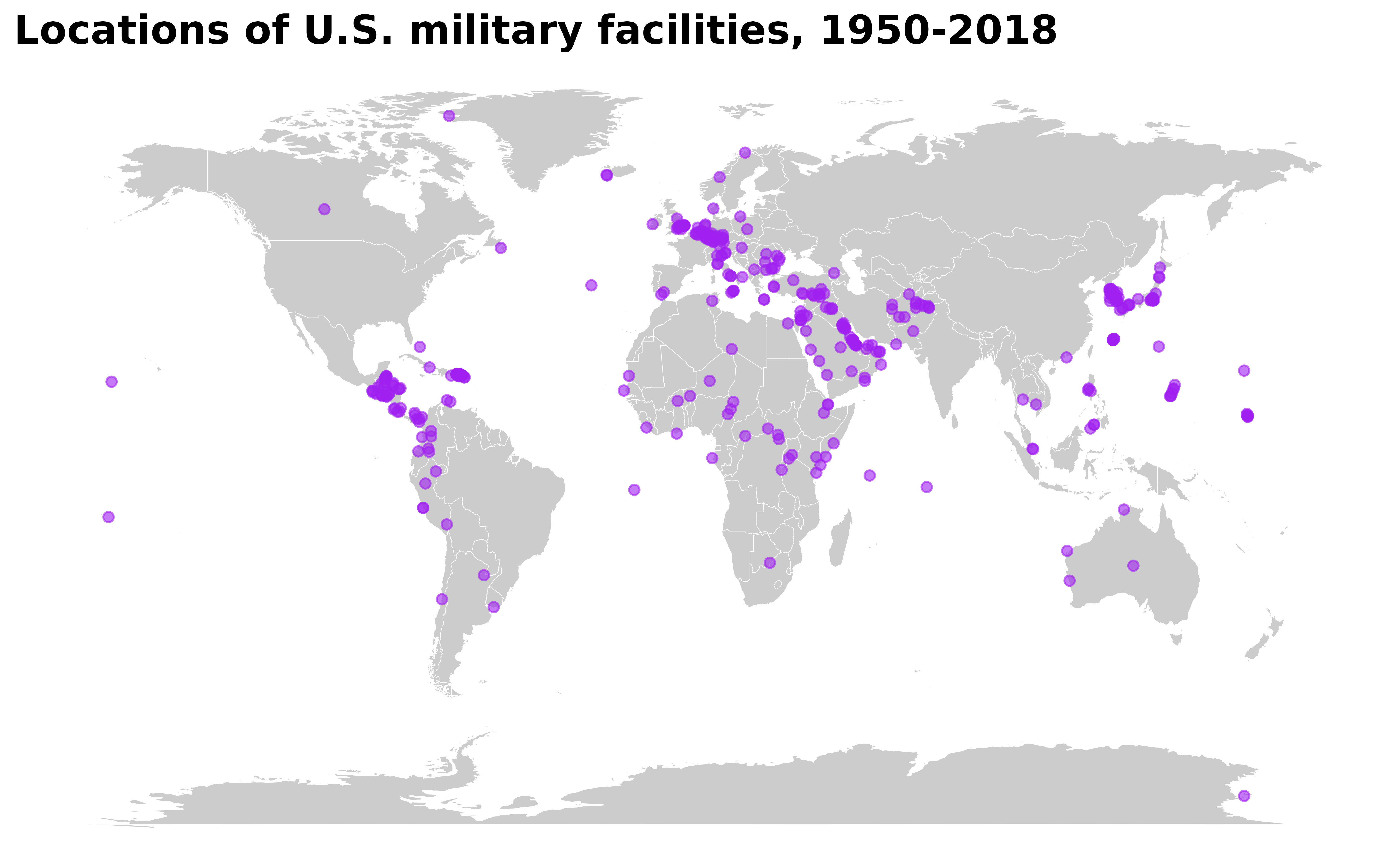
So what can you do with these super useful and cool data? Lots of things! The study of basing and military deployments has been picking up over the last few years and there are lots of cool studies you should check out. With these data you can do cool things like this!


library(ggplot2)

map <- ggplot2::map_data("world")
basepoints <- get_basedata(host = NA)


basemap <- ggplot() +
  geom_polygon(data = map, aes(x = long, y = lat, group = group), fill = "gray80", color = "white", size = 0.1) +
  geom_point(data = basepoints, aes(x = lon, y = lat), color = "purple", alpha = 0.6) +
  coord_equal(ratio = 1.3) +
  theme_void() +
  theme(plot.title = element_text(face = "bold", size = 15)) +
  labs(title = "Locations of U.S. military facilities, 1950-2018")


basemap